R Markdown

Introduction

R Markdown provides an unified authoring framework for data science, combining your code, its results, and your prose commentary. R Markdown documents are fully reproducible and support dozens of output formats, like PDFs, Word files, slideshows, and more.

R Markdown files are designed to be used in three ways:

1. For communicating to decision makers, who want to focus on the conclusions, not the code behind the analysis.

2. For collaborating with other data scientists (including future you!), who are interested in both your conclusions, and how you reached them (i.e. the code).

3. As an environment in which to do data science, as a modern day lab notebook where you can capture not only what you did, but also what you were thinking.

---

Prerequisites

You need the rmarkdown package, but you don’t need to explicitly install it or load it, as RStudio automatically does both when needed.

---

R Markdown basics

This is an R Markdown file, a plain text file that has the extension .Rmd:

It contains three important types of content:

1. An (optional) YAML header surrounded by ---s.
2. Chunks of R code surrounded by ```.
3. Text mixed with simple text formatting like # heading and _italics_.

---
title: "Diamond sizes"
date: 2016-08-25
output: html_document
---

```{r setup, include = FALSE}
library(ggplot2)
library(dplyr)

smaller <- diamonds %>% 
  filter(carat <= 2.5)
```

We have data about `r nrow(diamonds)` diamonds. Only 
`r nrow(diamonds) - nrow(smaller)` are larger than
2.5 carats. The distribution of the remainder is shown
below:

```{r, echo = FALSE}
smaller %>% 
  ggplot(aes(carat)) + 
  geom_freqpoly(binwidth = 0.01)
```

When you open an .Rmd, you get a notebook interface where code and output are interleaved. You can run each code chunk by clicking the Run icon (it looks like a play button at the top of the chunk), or by pressing Cmd/Ctrl + Shift + Enter. RStudio executes the code and displays the results inline with the code:

To produce a complete report containing all text, code, and results, click “Knit” or press Cmd/Ctrl + Shift + K. You can also do this programmatically with rmarkdown::render("1-example.Rmd"). This will display the report in the viewer pane, and create a self-contained HTML file that you can share with others.

When you knit the document R Markdown sends the .Rmd file to knitr, http://yihui.name/knitr/, which executes all of the code chunks and creates a new markdown (.md) document which includes the code and its output. The markdown file generated by knitr is then processed by pandoc, http://pandoc.org/, which is responsible for creating the finished file. The advantage of this two step workflow is that you can create a very wide range of output formats, as you’ll learn about in the section R markdown formats.

To get started with your own .Rmd file, select File > New File > R Markdown… in the menubar. RStudio will launch a wizard that you can use to pre-populate your file with useful content that reminds you how the key features of R Markdown work.

The following sections dive into the three components of an R Markdown document in more details: the markdown text, the code chunks, and the YAML header.

---

Text formatting with Markdown

Prose in .Rmd files is written in Markdown, a lightweight set of conventions for formatting plain text files. Markdown is designed to be easy to read and easy to write. It is also very easy to learn. The guide below shows how to use Pandoc’s Markdown, a slightly extended version of Markdown that R Markdown understands.

Text formatting 
------------------------------------------------------------

*italic*  or _italic_
**bold**   __bold__
`code`
superscript^2^ and subscript~2~

Headings
------------------------------------------------------------

# 1st Level Header

## 2nd Level Header

### 3rd Level Header

Lists
------------------------------------------------------------

*   Bulleted list item 1

*   Item 2

    * Item 2a

    * Item 2b

1.  Numbered list item 1

1.  Item 2. The numbers are incremented automatically in the output.

Links and images
------------------------------------------------------------

<http://example.com>

[linked phrase](http://example.com)

![optional caption text](path/to/img.png)

Tables 
------------------------------------------------------------

First Header  | Second Header
------------- | -------------
Content Cell  | Content Cell
Content Cell  | Content Cell

The best way to learn these is simply to try them out. It will take a few days, but soon they will become second nature, and you won’t need to think about them. If you forget, you can get to a handy reference sheet with Help > Markdown Quick Reference.

---

Code chunks

To run code inside an R Markdown document, you need to insert a chunk. There are three ways to do so:

1. The keyboard shortcut Cmd + Option + I

2. The “Insert” button icon in the editor toolbar.

3. By manually typing the chunk delimiters ```{r} and ```.

You can continue to run the code using the keyboard shortcut that by now you know and love: Cmd/Ctrl + Enter. However, chunks get a new keyboard shortcut: Cmd/Ctrl + Shift + Enter, which runs all the code in the chunk. Think of a chunk like a function. A chunk should be relatively self-contained, and focussed around a single task.

The following sections describe the chunk header which consists of ```{r, followed by an optional chunk name, followed by comma separated options, followed by }. Next comes your R code and the chunk end is indicated by a final ```.

Chunk name

Chunks can be given an optional name: ```{r by-name}. This has three advantages:

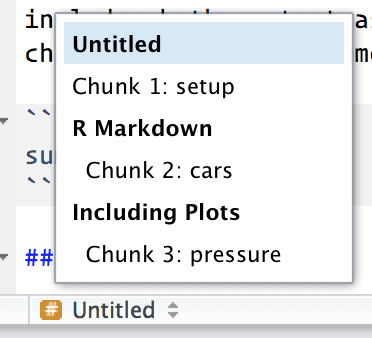
1. You can more easily navigate to specific chunks using the drop-down code navigator in the bottom-left of the script editor:

   

2. Graphics produced by the chunks will have useful names that make them easier to use elsewhere.

3. You can set up networks of cached chunks to avoid re-performing expensive computations on every run. More on that below.

There is one chunk name that imbues special behaviour: setup. When you’re in a notebook mode, the chunk named setup will be run automatically once, before any other code is run.

Chunk options

Chunk output can be customised with options, arguments supplied to chunk header. Knitr provides almost 60 options that you can use to customize your code chunks. Here we’ll cover the most important chunk options that you’ll use frequently. You can see the full list at http://yihui.name/knitr/options/.

The most important set of options controls if your code block is executed and what results are inserted in the finished report:

• eval = FALSE prevents code from being evaluated. (And obviously if the code is not run, no results will be generated). This is useful for displaying example code, or for disabling a large block of code without commenting each line.

• include = FALSE runs the code, but doesn’t show the code or results in the final document. Use this for setup code that you don’t want cluttering your report.

• echo = FALSE prevents code, but not the results from appearing in the finished file. Use this when writing reports aimed at people who don’t want to see the underlying R code.

• message = FALSE or warning = FALSE prevents messages or warnings from appearing in the finished file.

• results = 'hide' hides printed output; fig.show = 'hide' hides plots.

• error = TRUE causes the render to continue even if code returns an error. This is rarely something you’ll want to include in the final version of your report, but can be very useful if you need to debug exactly what is going on inside your .Rmd. It’s also useful if you’re teaching R and want to deliberately include an error. The default, error = FALSE causes knitting to fail if there is a single error in the document.

The following table summarises which types of output each option supressess:

Option	Run code	Show code	Output	Plots	Messages	Warnings
eval = FALSE	-		-	-	-	-
include = FALSE		-	-	-	-	-
echo = FALSE		-
results = "hide"			-
fig.show = "hide"				-
message = FALSE					-
warning = FALSE						-

---

Table

By default, R Markdown prints data frames and matrices as you’d see them in the console:

mtcars[1:5, ]

##                    mpg cyl disp  hp drat    wt  qsec vs am gear carb
## Mazda RX4         21.0   6  160 110 3.90 2.620 16.46  0  1    4    4
## Mazda RX4 Wag     21.0   6  160 110 3.90 2.875 17.02  0  1    4    4
## Datsun 710        22.8   4  108  93 3.85 2.320 18.61  1  1    4    1
## Hornet 4 Drive    21.4   6  258 110 3.08 3.215 19.44  1  0    3    1
## Hornet Sportabout 18.7   8  360 175 3.15 3.440 17.02  0  0    3    2

If you prefer that data be displayed with additional formatting you can use the knitr::kable function.

knitr::kable(
  mtcars[1:5, ], 
  caption = "A knitr kable."
)

A knitr kable.

	mpg	cyl	disp	hp	drat	wt	qsec	vs	am	gear	carb
Mazda RX4	21.0	6	160	110	3.90	2.620	16.46	0	1	4	4
Mazda RX4 Wag	21.0	6	160	110	3.90	2.875	17.02	0	1	4	4
Datsun 710	22.8	4	108	93	3.85	2.320	18.61	1	1	4	1
Hornet 4 Drive	21.4	6	258	110	3.08	3.215	19.44	1	0	3	1
Hornet Sportabout	18.7	8	360	175	3.15	3.440	17.02	0	0	3	2

Read the documentation for ?knitr::kable to see the other ways in which you can customise the table. For even deeper customisation, consider the xtable, stargazer, pander, tables, and ascii packages. Each provides a set of tools for returning formatted tables from R code.

There is also a rich set of options for controlling how figures are embedded.

---

Caching

Normally, each knit of a document starts from a completely clean state. This is great for reproducibility, because it ensures that you’ve captured every important computation in code. However, it can be painful if you have some computations that take a long time. The solution is cache = TRUE. When set, this will save the output of the chunk to a specially named file on disk. On subsequent runs, knitr will check to see if the code has changed, and if it hasn’t, it will reuse the cached results.

Global options

As you work more with knitr, you will discover that some of the default chunk options don’t fit your needs and you want to change them. You can do this by calling knitr::opts_chunk$set() in a code chunk. For example, when writing books and tutorials I set:

knitr::opts_chunk$set(
  comment = "#>",
  collapse = TRUE
)

This ensures that the code and output are kept closely entwined. On the other hand, if you were preparing a report, you might set:

knitr::opts_chunk$set(
  echo = FALSE
)

That will hide the code by default, so only showing the chunks you deliberately choose to show (with echo = TRUE). You might consider setting message = FALSE and warning = FALSE, but that would make it harder to debug problems because you wouldn’t see any messages in the final document.

---

Inline code

There is one other way to embed R code into an R Markdown document: directly into the text, with: `r `. This can be very useful if you mention properties of your data in the text. For example, in the example document I used at the start of the chapter I had:

We have data about `r nrow(diamonds)` diamonds. Only `r nrow(diamonds) - nrow(smaller)` are larger than 2.5 carats. The distribution of the remainder is shown below:

When the report is knit, the results of these computations are inserted into the text:

We have data about 53940 diamonds. Only 126 are larger than 2.5 carats. The distribution of the remainder is shown below:

When inserting numbers into text, format() is your friend. It allows you to set the number of digits so you don’t print to a ridiculous degree of accuracy, and a big.mark to make numbers easier to read. I’ll often combine these into a helper function:

comma <- function(x) format(x, digits = 2, big.mark = ",")
comma(3452345)

## [1] "3,452,345"

comma(.12358124331)

## [1] "0.12"

---

The YAML “yet another markup language” header

You can control many other “whole document” settings by tweaking the parameters of the YAML header. YAML stands for: it’s “yet another markup language”, which is designed for representing hierarchical data in a way that’s easy for humans to read and write. R Markdown uses it to control many details of the output. Here we’ll discuss two: document parameters and bibliographies.

---

Parameters

R Markdown documents can include one or more parameters whose values can be set when you render the report.

Parameters are useful when you want to re-render the same report with distinct values for various key inputs. For example, you might be producing sales reports per branch, exam results by student, or demographic summaries by country. To declare one or more parameters, use the params field.

This example use a my_class parameter to determines which class of cars to display:

---
output: html_document
params:
  my_class: "suv"
---

```{r setup, include = FALSE}
library(ggplot2)
library(dplyr)

class <- mpg %>% filter(class == params$my_class)
```

# Fuel economy for `r params$my_class`s

```{r, message = FALSE}
ggplot(class, aes(displ, hwy)) + 
  geom_point() + 
  geom_smooth(se = FALSE)
```

Bibliographies and Citations

Pandoc can automatically generate citations and a bibliography in a number of styles. To use this feature, specify a bibliography file using the bibliography field in your file’s header. The field should contain a path from the directory that contains your .Rmd file to the file that contains the bibliography file:

bibliography: rmarkdown.bib

You can use many common bibliography formats including BibLaTeX, BibTeX, endnote, medline.

To create a citation within your .Rmd file, use a key composed of ‘@’ + the citation identifier from the bibliography file. Then place the citation in square brackets. Here are some examples:

Separate multiple citations with a `;`: Blah blah [@smith04; @doe99].

You can add arbitrary comments inside the square brackets: 
Blah blah [see @doe99, pp. 33-35; also @smith04, ch. 1].

Remove the square brackets to create an in-text citation: @smith04 
says blah, or @smith04 [p. 33] says blah.

Add a `-` before the citation to suppress the author's name: 
Smith says blah [-@smith04].

When R Markdown renders your file, it will build and append a bibliography to the end of your document. The bibliography will contain each of the cited references from your bibliography file, but it will not contain a section heading. As a result it is common practice to end your file with a section header for the bibliography, such as # References or # Bibliography.

You can change the style of your citations and bibliography by referencing a CSL (citation style language) file in the csl field:

bibliography: rmarkdown.bib
csl: apa.csl

As with the bibliography field, your csl file should contain a path to the file. Here I assume that the csl file is in the same directory as the .Rmd file. A good place to find CSL style files for common bibliography styles is http://github.com/citation-style-language/styles.

A work by Matteo Cereda and Fabio Iannelli