Data structure in R
R provides basic and advanced data structure that can be used
to store your information:
| Level | Data types |
|---|---|
Beginner |
Vector, Matrix, List, Dataframe |
Pro |
S3, S4, RC |
R’s basic data structures can be organised by their dimensionality whether they’re:
- homogeneous (all contents must be of the same type) or
- heterogeneous (the contents can be of different types).
This gives rise to the five data types most often used in data analysis:
| Dimensions | Homogeneous | Heterogeneous |
|---|---|---|
| 1 | Atomic vector | List |
| 2 | Matrix | Data frame |
| n | Array |
R has no 0-dimensional, or scalar, types.
Individual numbers or strings, which you might think would be scalars, are vectors of length one.
Vectors
There are two types of vectors:
Atomic
of which there are 6 types:
| 1. | logical | |
| 2. | integer | |
| 3. | double | integer and double vectors are collectively known as numeric vectors |
| 4. | complex | complex number |
| 5. | character | |
| 6. | raw | intended to hold raw bytes |
Lists
which are sometimes called recursive vectors because lists can contain other lists.
The main difference between atomic vectors and lists is that atomic vectors are homogeneous, while lists can be heterogeneous.
Every vector has two key properties:
Its TYPE, which you can determine with
typeof().cat(" 10 is a", typeof(10), "\n");## 10 is a doubleLETTERS; typeof(LETTERS);## [1] "A" "B" "C" "D" "E" "F" "G" "H" "I" "J" "K" "L" "M" "N" "O" "P" "Q" "R" "S" "T" "U" ## [22] "V" "W" "X" "Y" "Z"## [1] "character"Its LENGTH, which you can determine with
length().x <- list("a", "b", 1:10) length(x)## [1] 3
 There’s one other
related object:
There’s one other
related object:
The NULL object
NULLis often used to represent the absence of a vector (as opposed toNAwhich is used to represent the absence of a value in a vector).NULLtypically behaves like a vector of length 0.
The relationships between vectors can be summised as follows:
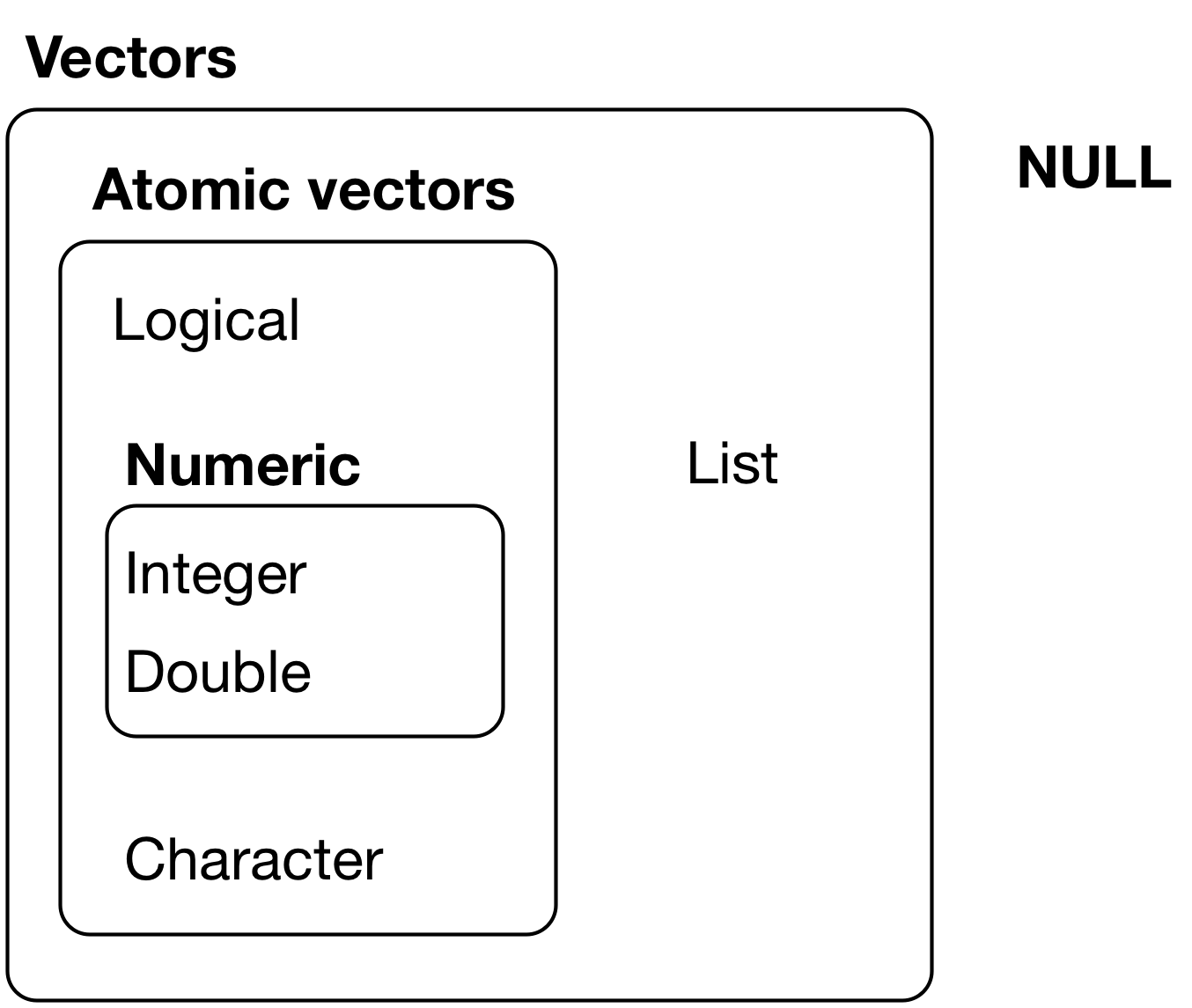
The hierarchy of R’s vector types
Creation of a vector
Constructor
A vector can be easily defined using the function c()
(“concatenate”)
# Create a vector x of size 4 and allocate the elements
x <- c(1,4,3,4)
print(x)
## [1] 1 4 3 4 Watch out:
in R vectors are 1-based
meaning that x[1] will return your first vector element.
print(x[1]) ## [1] 1Concatenation
Vectors can be joined together using c()
a <- c(1, -2.4)
b <- c(47, 52)
x <- c(a, b, -80)
print(x)
## [1] 1.0 -2.4 47.0 52.0 -80.0Operations with vectors
Add/Multiply a number to a vector
x = 5 + c(10, 20)
print(x)
## [1] 15 25Add two vectors of the same length
x = c(-1, 5, -10) + c(5, 5, 10)
print(x)
## [1] 4 10 0Apply a function to each element of a vector
x = log10(c(10,100,1000))
print(x)
## [1] 1 2 3Operations with recycling
Two vectors of the same length are added/subtracted/multiplied/divided in a elementwise manner
x = c(1,5) + c(10, 20)
print(x)
## [1] 11 25 Watch out:
If vectors have different lengths, the shorter is recycled
and you will likely get a warning message
x = c(1, 5) + c(5, 5, 10)## Warning in c(1, 5) + c(5, 5, 10): longer object length is not a multiple of shorter object
## lengthprint(x)## [1] 6 10 11Indexing
Vector elements can be accessed using the brackets [ ]
in different ways.
# Suppose we have this named vectors:
x = c(1, 2, 3, 4)
names(x) = c("a", "b", "c", "d")| Mode | Code | |
|---|---|---|
| 1. | Position | x[c(1,4)] |
| 2. | Selection | x[c(T,F,F,T)] |
| 3. | All positions except some | x[-c(2,3)] |
| 4. | Names | x[c("a","d")] |
Here we are:
#1.
x[c(1,4)]
## a d
## 1 4#2.
x[c(T,F,F,T)]## a d
## 1 4#3.
x[-c(2,3)]## a d
## 1 4#4.
x[c("a","d")]## a d
## 1 4You can select entries several times:
x[c(1,1,1,4,4,4)]## a a a d d d
## 1 1 1 4 4 4| Functions for selection |
|---|
which() |
%in% |
match() |
grep() |
grepl() |
To select elements that satisfy a logic condition you can use the
function which()
x = c(1,2,3,4);

which(x>2)
## [1] 3 4Other functions : %in%, match(),
grep()
x = c("a","b","c","d");

x %in% c("b","c")
## [1] FALSE TRUE TRUE FALSEmatch(x, c("b","c") ) ## [1] NA 1 2 NAgrep(c("b","c"), x ) ## Warning in grep(c("b", "c"), x): argument 'pattern' has length > 1 and only the first
## element will be used## [1] 2What’s inside?
How a vector is internally implemented in R?
To see it you can use the function str().
str() display the internal structure of an R object. It
is a diagnostic function.
v = c( x=1, y=2, z=3 );
# What's inside?
str(v)
## Named num [1:3] 1 2 3
## - attr(*, "names")= chr [1:3] "x" "y" "z"v is a numeric vector with 3 elements and an attribute called names.
Attributes can be retrieved and set using the attr()
function.
attr(v,"names")## [1] "x" "y" "z"Attributes
Any vector can contain arbitrary additional metadata through its attributes, or metadata.
You can think of attributes as named list of vectors that can be attached to any object.
You can:
get and set individual attribute values with
attr()see them all at once with
attributes().
x <- 1:10
#setting attributes
attr(x, "greeting")
## NULLattr(x, "greeting") <- "Hi!"
attr(x, "farewell") <- "Bye!"# Check attributes
attributes(x)## $greeting
## [1] "Hi!"
##
## $farewell
## [1] "Bye!" There are three
very important attributes that are used to implement
fundamental parts of R:
Names are used to name the elements of a vector.
Dimensions make a vector behave like a matrix or array.
Class is used to implement the S3 object oriented system.
Data types
Elements of a vector must be of the same type.
We can not combine, numerical values, character strings and logicals in the same vector. If we try, values are coerced.
x <- c("Breakin","rocks","in","the","hot","sun")
typeof(x)
## [1] "character"x <- c("Breakin","rocks","in","the","hot","sun", "take", 2)
typeof(x)## [1] "character"x## [1] "Breakin" "rocks" "in" "the" "hot" "sun" "take" "2"Numeric
Integer and double vectors are known collectively as numeric vectors.
In R, numbers are doubles by default.
To make an integer, place an L after the number:
typeof(1)## [1] "double"typeof(1L)## [1] "integer"1.5L## [1] 1.5The distinction between integers and doubles is not usually important, but there are two important differences that you should be aware of:
- Doubles are approximations.
Doubles represent floating point numbers that can not always be precisely represented with a fixed amount of memory. This means that you should consider all doubles to be approximations.
For example, what is square of the square root of two?
x <- sqrt(2) ^ 2
x
## [1] 2x - 2## [1] 4.440892e-16This behaviour is common when working with floating point numbers: most calculations include some approximation error.
Instead of comparing floating point numbers using
==, you should usedplyr::near()which allows for some numerical tolerance.
- Integers have 1 special value:
NA, while doubles have 4:NA,NaN,Infand-Inf.
| Numeric | Special values |
|---|---|
| Integers | NA |
| Double | NA, NaN, Inf and
-Inf |
All three special values NaN, Inf and
-Inf can arise in during division:
c(-1, 0, 1) / 0## [1] -Inf NaN InfAvoid using == to check for these other special values.
Instead use the helper functions is.finite(),
is.infinite(), and is.nan():
| 0 | Inf | NA | NaN | |
|---|---|---|---|---|
is.finite() |
 |
|||
is.infinite() |
|
|||
is.na() |
|
|
||
is.nan() |
|
Character
Character vectors are the most complex type of atomic vector.
R uses a global string pool.
This means that each unique string is only stored in memory once, and every use of the string points to that representation.
This reduces the amount of memory needed by duplicated strings.
You can see this behavior in practice with
pryr::object_size():
x <- "This is a reasonably long string."
pryr::object_size(x)
## 152 By <- rep(x, 1000)
pryr::object_size(y)## 8,144 By doesn’t take up 1,000x as much memory as
x, because each element of y is just a pointer
to that same string. A pointer is ~8 bytes, so 1000 pointers to a 152 B
string is 8 * 1000 + 152 = 8.14 kB.
Factors
Factors are designed to represent categorical data that can take a fixed set of possible values.
Factors are built on top of integers, and have a levels attribute:
x <- factor( c("ab", "cd", "ab"), levels = c("ab", "cd", "ef") )
typeof(x)
## [1] "integer"attributes(x)## $levels
## [1] "ab" "cd" "ef"
##
## $class
## [1] "factor"Internally, a factor is a numeric vector but to each value of the
vector there is associated a level.
levels(x)## [1] "ab" "cd" "ef"Missing Values
Missing values are indicated by NA. To select the
non-missing values in a vector do:
v = c(NA,5,10)
v[!is.na(v)]
## [1] 5 10# to return indexes of non-missing values
which(!is.na(v)) ## [1] 2 3Logical values (+ operators)
A logical expression is an expression which is either
TRUE or FALSE (abbreviated as T and F in
R).
Logical operators are the usual ones (==,!,
>, <, &, |
).
The operator & and && (or
| and ||) have different behavior with
arrays.
The shorter form performs ELEMENTWISE comparisons in much the same way as arithmetic operators.
The longer form evaluates left to right examining ONLY the FIRST element of each vector.
my_vector = c(1,2)

my_vector==1 & my_vector>0 # SHORT
## [1] TRUE FALSEmy_vector==1 && my_vector>0 # SHORT LONG## [1] TRUECoercion
“the practice of persuading someone to do something by using force or threats”
There are two ways to convert one type of vector to another:
Explicit coercion happens when you call a function like
as.logical(),as.integer(),as.double(), oras.character().Implicit coercion happens when you use a vector in a specific context that expects a certain type of vector. For example, the most important type of implicit coercion: using a logical vector in a numeric context. In this case
TRUEis converted to1andFALSEconverted to 0. That means the sum of a logical vector is the number ofTRUEs, and the mean of a logical vector is the proportion ofTRUEs:
x <- sample(20, 100, replace = TRUE)
y <- x > 10
sum(y)  # how many are greater than 10?
## [1] 52mean(y) # what proportion are greater than 10?## [1] 0.52You may see some code that relies on implicit coercion in the opposite direction, from integer to logical:
if (length(x)) {
  # do something
}
In this case, 0 is converted to FALSE and everything
else is converted to TRUE.
This makes it harder to understand your code, and I don’t recommend
it. Instead be explicit: length(x) > 0.
when you create a vector containing multiple types with
c(): the most complex type always wins.
typeof(c(TRUE, 1L))## [1] "integer"typeof(c(1.5, "a"))## [1] "character"An atomic vector can not have a mix of different types because the type is a property of the complete vector, not the individual elements. If you need to mix multiple types in the same vector, you should use a list.
Test functions
Sometimes you want to do different things based on the type of vector.
One option is to use typeof().
Another is to use a test function which returns a TRUE
or FALSE.
Base R provides many functions like is.vector() and
is.atomic(). However, the purr package provide a more
comprehensive list of teste function, which are summarised in the table
below.
| lgl | int | dbl | chr | list | |
|---|---|---|---|---|---|
is_logical() |
|
||||
is_integer() |
|
||||
is_double() |
|
||||
is_numeric() |
|
|
|||
is_character() |
|
||||
is_atomic() |
|
|
|
|
|
is_list() |
|
||||
is_vector() |
|
|
|
|
|
Generating sequences
Sequence by repetition
rep( c(10, 20, 30), times = 4)## [1] 10 20 30 10 20 30 10 20 30 10 20 30Sequence of equally spaced numbers
seq(from = 0, to = 5, lenght.out = 4)## [1] 0 1 2 3 4 5seq(from = 0, to = 5, by = 1.25)## [1] 0.00 1.25 2.50 3.75 5.00Generate random data from Uniform distribution
unif = runif(n = 100)
hist(unif,10)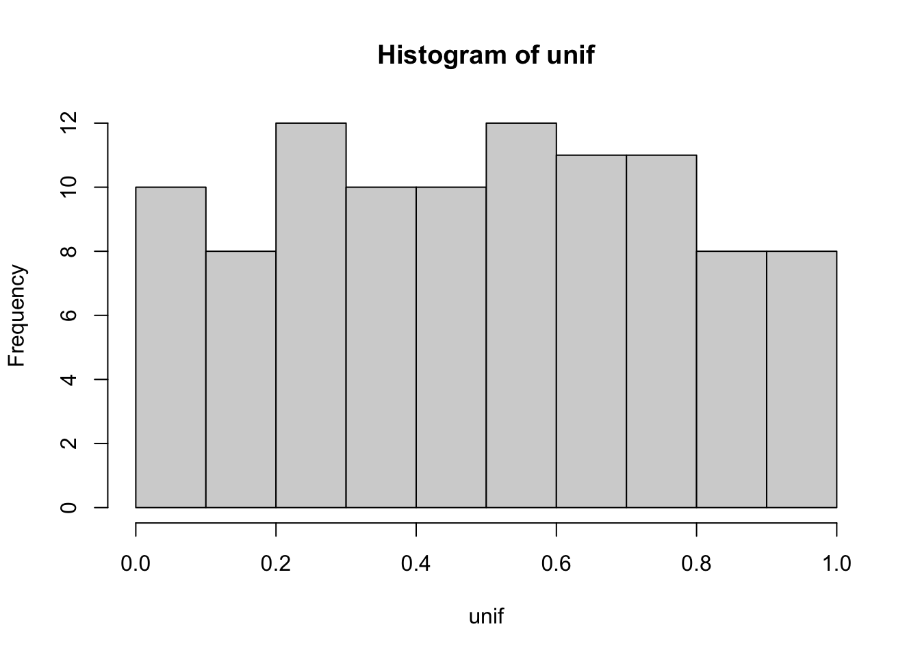
Generate random data from Normal distribution
norm = rnorm(n = 100, mean = 5, sd = 0.1)
hist(norm)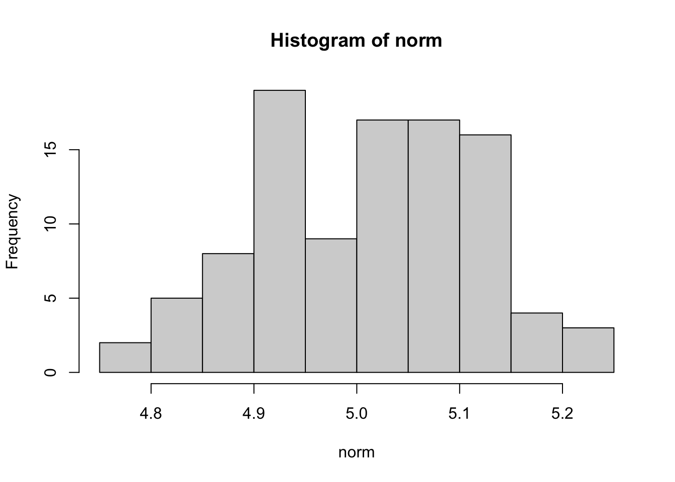
Generate random data from Negative Bimodal distribution
nb = rnbinom(n = 100, mu = 5, size = 1/0.1)
hist(nb)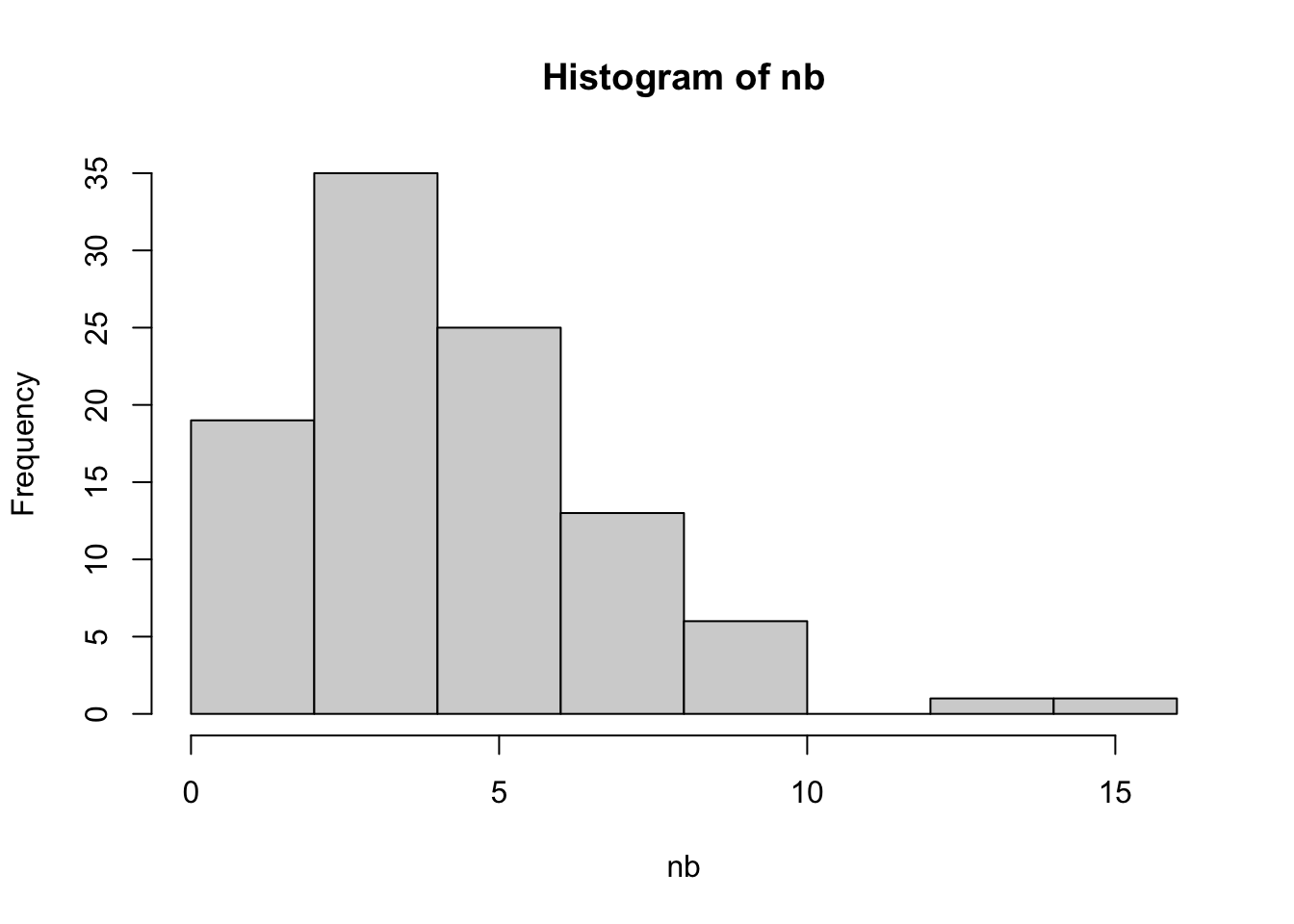
But I guess that some of you have already seen these distribution in the previous course

Please don't
Matrices
Matrices are created with the function matrix()
m = matrix( data = 1:4, nrow=2, ncol=2, byrow=T )
str(m)
## int [1:2, 1:2] 1 3 2 4A matrix is basically a vector with a dimension attribute.
dim(m)## [1] 2 2dim(m) = c(1,4); # change matrix dimension
m## [,1] [,2] [,3] [,4]
## [1,] 1 3 2 4m = 1:4 ;
dim(m) = c(2,2); #from "vector" to "matrix
m## [,1] [,2]
## [1,] 1 3
## [2,] 2 4Matrices can be created by converting a vector into a matrix or by binding together vectors
#from a vector
as.matrix(c(1,2))## [,1]
## [1,] 1
## [2,] 2# binding 2 vectors by rows
rbind(x=1:3,y=4:6)## [,1] [,2] [,3]
## x 1 2 3
## y 4 5 6# binding 2 vectors by rows
cbind(x=1:3,y=4:6)## x y
## [1,] 1 4
## [2,] 2 5
## [3,] 3 6The transposed matrix
matrix(1:4,nr=2,nc=2,byrow=T)## [,1] [,2]
## [1,] 1 2
## [2,] 3 4#Traspose it
t(matrix(1:4,nr=2,nc=2,byrow=T))## [,1] [,2]
## [1,] 1 3
## [2,] 2 4The diagonal matrix
diag(c(1,2,3),nr=3,nc=4)## [,1] [,2] [,3] [,4]
## [1,] 1 0 0 0
## [2,] 0 2 0 0
## [3,] 0 0 3 0The triangular matrix
m = matrix(1:6,nr=3,nc=3,byrow=T)
m## [,1] [,2] [,3]
## [1,] 1 2 3
## [2,] 4 5 6
## [3,] 1 2 3tri = lower.tri(m, diag = FALSE)
m[tri] = NA
m## [,1] [,2] [,3]
## [1,] 1 2 3
## [2,] NA 5 6
## [3,] NA NA 3tri = upper.tri(m, diag = TRUE)
m[tri] = 1
m## [,1] [,2] [,3]
## [1,] 1 1 1
## [2,] NA 1 1
## [3,] NA NA 1Indexing
For a matrix m, the value of the i-th row and j-th
column is accessed with mat[i, j]
m = matrix(1:4,nr=2,nc=2);
m## [,1] [,2]
## [1,] 1 3
## [2,] 2 4m[ c(1,2), 2 ]## [1] 3 4Indexing can be used to suppress rows and/or columns.
m = matrix(1:4,nr=2,nc=2);
m## [,1] [,2]
## [1,] 1 3
## [2,] 2 4# get rid of second column
m[,-2]## [1] 1 2m = matrix(1:4,nr=2,nc=2);
m## [,1] [,2]
## [1,] 1 3
## [2,] 2 4dimnames(m)=list(NULL,c("a","b"))
m[,"a"]## [1] 1 2Operations
Standard operations on matrices are element by element.
matrix(c(1,2),nr=2) + matrix(c(1,3),nr=2)## [,1]
## [1,] 2
## [2,] 5matrix(c(1,2),nr=2) * matrix(c(1,3),nr=2)## [,1]
## [1,] 1
## [2,] 6
Matrices must be consistent, of the same dimensions
otherwise you will get this error:
Error in matrix(2, nr = 2, nc = 2) + matrix(c(1, 3), nc = 2) :
non-conformable arraysComing back to this operation:
matrix(c(1,2),nr=2) * matrix(c(1,3),nr=2)## [,1]
## [1,] 1
## [2,] 6This is not the matrix product, the matrix multiplication looks like:
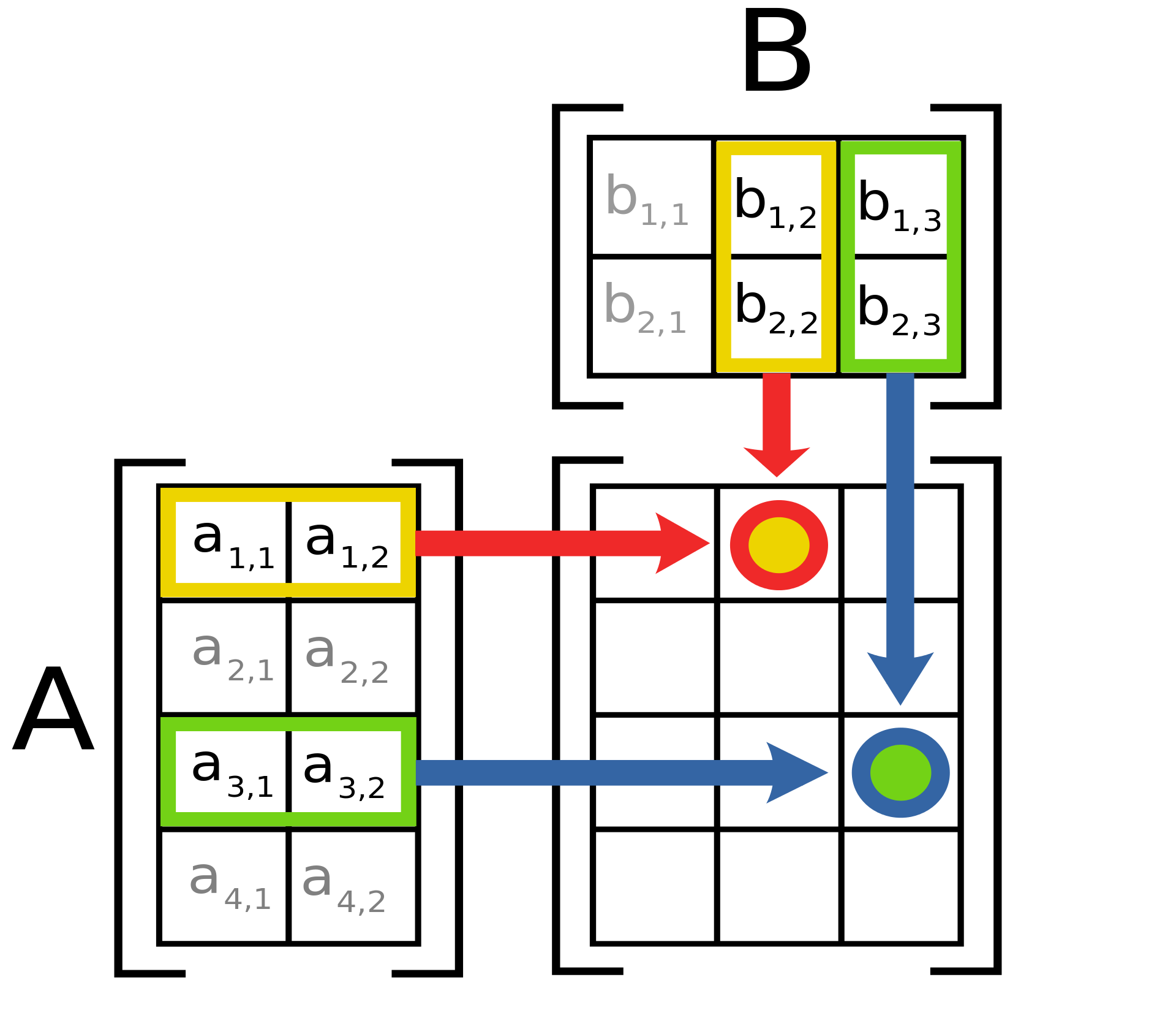

Matrix multiplication
The operator for matrix multiplication is
%*%.
x=diag(c(1,2)); x;## [,1] [,2]
## [1,] 1 0
## [2,] 0 2y = matrix(1:6, ncol = 3, nrow = 2); y;## [,1] [,2] [,3]
## [1,] 1 3 5
## [2,] 2 4 6# Let't check the matrix multiplation
x%*%y## [,1] [,2] [,3]
## [1,] 1 3 5
## [2,] 4 8 12In a matrix product between a vector and a matrix, the vector is
interpreted as row vector for vector %*% matrix and is
interpreted as column vector for matrix %*% vector. The
convention for vector %*% vector is to interpret the
product as scalar product rowvector %*% columnvector.
Lists
Lists are heterogenoues collections of arbitrary
objects created with the function list()
list( array=c(1,5,3)
, matrix=matrix(1:4, nrow=2)
, person=c(name="Stacy", surname="Peralta")
)## $array
## [1] 1 5 3
##
## $matrix
##      [,1] [,2]
## [1,]    1    3
## [2,]    2    4
##
## $person
## name surname
## "Stacy" "Peralta"
The elements of a list can be of different types and lengths.
It is often convenient to name the elements of a list.
To save time and space you can printout a list using
str()
str( list( array=c(1,5,3), matrix=matrix(1:4, nrow=2), person=c(name="Stacy", surname="Peralta") ) )## List of 3
## $ array : num [1:3] 1 5 3
## $ matrix: int [1:2, 1:2] 1 2 3 4
## $ person: Named chr [1:2] "Stacy" "Peralta"
## ..- attr(*, "names")= chr [1:2] "name" "surname"Indexing
l = list( array=c(1,5,3)
, matrix=matrix(1:4, nrow=2)
, person=c(name="Stacy", surname="Peralta")
)
l## $array
## [1] 1 5 3
##
## $matrix
##      [,1] [,2]
## [1,]    1    3
## [2,]    2    4
##
## $person
## name surname
## "Stacy" "Peralta"## Selection
l[c(T,F,T)] # l[c(1,3)]## $array
## [1] 1 5 3
##
## $person
## name surname
## "Stacy" "Peralta"## Element
l[["matrix"]]; l[2]## [,1] [,2]
## [1,] 1 3
## [2,] 2 4## $matrix
##      [,1] [,2]
## [1,]    1    3
## [2,] 2 4[["matrix"]]extracts the contents of the “matrix” element of list.[2]extracts the list consisting of the “matrix” element of list.
Concatenation
Lists can be concatenated using the function c()
c( list( array=c(1,5,3)
, matrix=matrix(1:4, nrow=2)),
list(person=c(name="Stacy", surname="Peralta") ) )## $array
## [1] 1 5 3
##
## $matrix
##      [,1] [,2]
## [1,]    1    3
## [2,]    2    4
##
## $person
## name surname
## "Stacy" "Peralta"Dataframes
A dataframe is a rectangular array where columns can be integers, numericals, characters, factors and other types of data.
It is essentially a list in which all elements have the same length.
d = data.frame(  id = 1:6
               , type = c(rep("T",3),rep("U",3)),
                 score = runif(6));
d
## id type score
## 1 1 T 0.06834669
## 2 2 T 0.60194281
## 3 3 T 0.71802842
## 4 4 U 0.34562478
## 5 5 U 0.58856669
## 6 6 U 0.71187147colnames(d)## [1] "id" "type" "score"rownames(d) = paste("chr",1:6,sep="",coll="") ;
rownames(d)## [1] "chr1" "chr2" "chr3" "chr4" "chr5" "chr6"Indexing
Indexed as a matrix.
A specific variables (columns) can be extracted using
[[ ]]or$as
d = data.frame(  id = 1:6
               , type = c(rep("T",3),rep("U",3)),
                 score = runif(6))

d[["score"]]
## [1] 0.78654326 0.06390668 0.53102870 0.97671334 0.77794910 0.75319486Select rows of a dataframe for certain values of some column variables. Let’s select a subset of the rows for which state is treated and score>0.6
idx = d$type=='T' & d$score > 0.6
idx
## [1] TRUE FALSE FALSE FALSE FALSE FALSEd[idx, c('id','type')]## id type
## 1 1 TAdding/removing variables
Suppose we want to add a new variable to the dataframe. One way is as follows:
d$value = NA
head(d, 2)
## id type score value
## 1 1 T 0.78654326 NA
## 2 2 T 0.06390668 NAd$value = floor(d$score*100);
head(d, 2)## id type score value
## 1 1 T 0.78654326 78
## 2 2 T 0.06390668 6d$value = NULL;
head(d, 2)## id type score
## 1 1 T 0.78654326
## 2 2 T 0.06390668A work by Matteo Cereda and Fabio Iannelli