Tidy the data

Prerequisites

Here we’ll focus on tidyr, a package that provides a bunch of tools to help tidy up your messy datasets.

suppressWarnings(library(tidyverse))

---

Tidy data

You can represent the same underlying data in multiple ways.

The example below shows the same data organised in four different ways. Each dataset shows the same values of four variables country, year, population, and cases, but each dataset organises the values in a different way.

table1

## # A tibble: 6 × 4
##   country      year  cases population
##   <chr>       <int>  <int>      <int>
## 1 Afghanistan  1999    745   19987071
## 2 Afghanistan  2000   2666   20595360
## 3 Brazil       1999  37737  172006362
## 4 Brazil       2000  80488  174504898
## 5 China        1999 212258 1272915272
## 6 China        2000 213766 1280428583

table2

## # A tibble: 12 × 4
##    country      year type            count
##    <chr>       <int> <chr>           <int>
##  1 Afghanistan  1999 cases             745
##  2 Afghanistan  1999 population   19987071
##  3 Afghanistan  2000 cases            2666
##  4 Afghanistan  2000 population   20595360
##  5 Brazil       1999 cases           37737
##  6 Brazil       1999 population  172006362
##  7 Brazil       2000 cases           80488
##  8 Brazil       2000 population  174504898
##  9 China        1999 cases          212258
## 10 China        1999 population 1272915272
## 11 China        2000 cases          213766
## 12 China        2000 population 1280428583

table3

## # A tibble: 6 × 3
##   country      year rate             
## * <chr>       <int> <chr>            
## 1 Afghanistan  1999 745/19987071     
## 2 Afghanistan  2000 2666/20595360    
## 3 Brazil       1999 37737/172006362  
## 4 Brazil       2000 80488/174504898  
## 5 China        1999 212258/1272915272
## 6 China        2000 213766/1280428583

# Spread across two tibbles
table4a  # cases

## # A tibble: 3 × 3
##   country     `1999` `2000`
## * <chr>        <int>  <int>
## 1 Afghanistan    745   2666
## 2 Brazil       37737  80488
## 3 China       212258 213766

table4b  # population

## # A tibble: 3 × 3
##   country         `1999`     `2000`
## * <chr>            <int>      <int>
## 1 Afghanistan   19987071   20595360
## 2 Brazil       172006362  174504898
## 3 China       1272915272 1280428583

These are all representations of the same underlying data, but they are not equally easy to use.

One dataset, the tidy dataset, will be much easier to work with inside the tidyverse.

There are three interrelated rules which make a dataset tidy:

1. Each variable must have its own column.

2. Each observation must have its own row.

3. Each value must have its own cell.

Figure shows the rules visually.

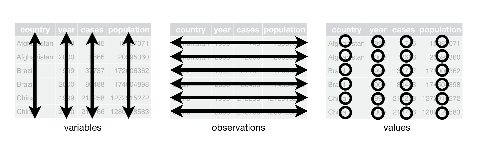
Following three rules makes a dataset tidy: variables are in columns, observations are in rows, and values are in cells.

These three rules are interrelated because it’s impossible to only satisfy two of the three.

In this example, only table1 is tidy. It’s the only representation where each column is a variable.

Why ensure that your data is tidy?

There are two main advantages:

1. There’s a general advantage to picking one consistent way of storing data. If you have a consistent data structure, it’s easier to learn the tools that work with it because they have an underlying uniformity.

2. There’s a specific advantage to placing variables in columns because it allows R’s vectorised nature to shine.

dplyr, ggplot2, and all the other packages in the tidyverse are designed to work with tidy data.

Here are a couple of small examples showing how you might work with table1.

# Compute rate per 10,000
table1 %>% 
  mutate(rate = cases / population * 10000)

## # A tibble: 6 × 5
##   country      year  cases population  rate
##   <chr>       <int>  <int>      <int> <dbl>
## 1 Afghanistan  1999    745   19987071 0.373
## 2 Afghanistan  2000   2666   20595360 1.29 
## 3 Brazil       1999  37737  172006362 2.19 
## 4 Brazil       2000  80488  174504898 4.61 
## 5 China        1999 212258 1272915272 1.67 
## 6 China        2000 213766 1280428583 1.67

# Compute cases per year
table1 %>% 
  count(year, wt = cases)

## # A tibble: 2 × 2
##    year      n
##   <int>  <int>
## 1  1999 250740
## 2  2000 296920

---

Spreading and gathering

The first step is always to: figure out what the variables and observations are.

The second step is to solve one of two common problems:

1. One variable might be spread across multiple columns.

2. One observation might be scattered across multiple rows.

To fix these problems, you’ll need the two most important functions in tidyr:

• gather()

• spread()

---

gather()

A common problem is a dataset where:

some of the column names are NOT names of variables RATHER observations/values of a variable themselves.

Take table4a: the column names 1999 and 2000 represent values of the year variable, and each row represents two observations, not one.

table4a

## # A tibble: 3 × 3
##   country     `1999` `2000`
## * <chr>        <int>  <int>
## 1 Afghanistan    745   2666
## 2 Brazil       37737  80488
## 3 China       212258 213766

To tidy a dataset like this, we need to gather those columns into a new pair of variables.

To describe that operation we need three parameters:

1. The set of columns that represent values, not variables.

2. The name of the variable whose values form the column names. I call that the key, and here it is year.

3. The name of the variable whose values are spread over the cells. I call that value, and here it’s the number of cases.

table4a %>% 
  gather(`1999`, `2000`, key = "year", value = "cases")

## # A tibble: 6 × 3
##   country     year   cases
##   <chr>       <chr>  <int>
## 1 Afghanistan 1999     745
## 2 Brazil      1999   37737
## 3 China       1999  212258
## 4 Afghanistan 2000    2666
## 5 Brazil      2000   80488
## 6 China       2000  213766

Here there are only two columns, so we list them individually. Note that “1999” and “2000” are non-syntactic names so we have to surround them in backticks.

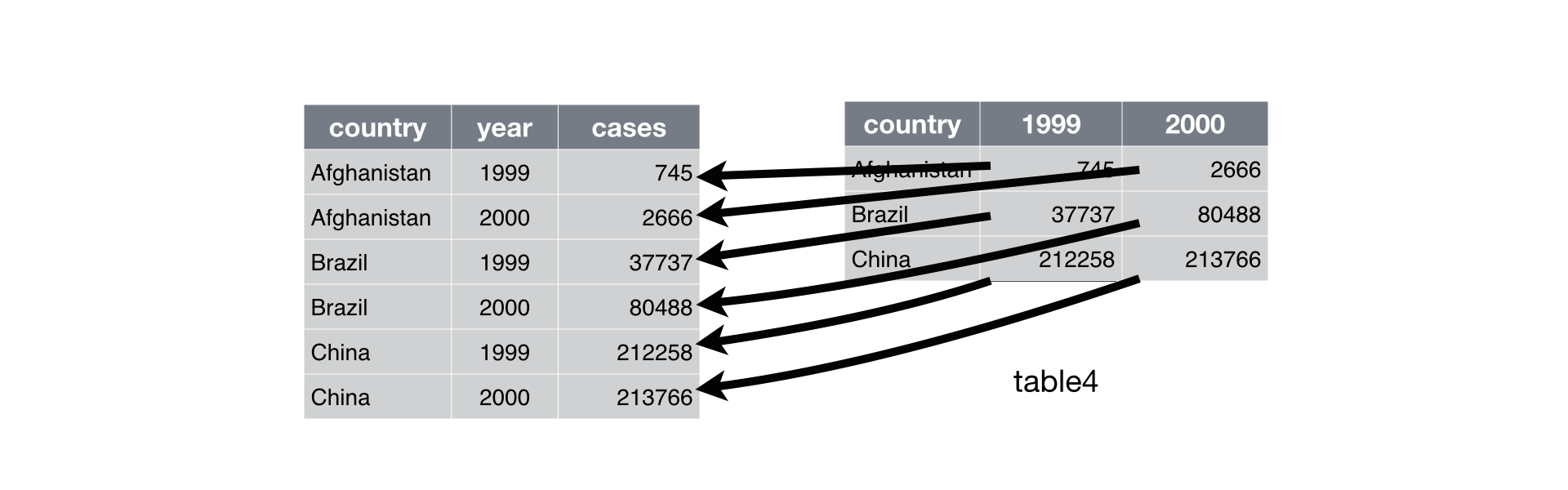
Gathering table4 into a tidy form.

table4b %>% 
  gather(`1999`, `2000`, key = "year", value = "population")

## # A tibble: 6 × 3
##   country     year  population
##   <chr>       <chr>      <int>
## 1 Afghanistan 1999    19987071
## 2 Brazil      1999   172006362
## 3 China       1999  1272915272
## 4 Afghanistan 2000    20595360
## 5 Brazil      2000   174504898
## 6 China       2000  1280428583

• To combine the tidied versions of table4a and table4b into a single tibble, we need to use dplyr::left_join()

# gather table a
tidy4a <- table4a %>% gather(`1999`, `2000`, key = "year", value = "cases")
# gather table b
tidy4b <- table4b %>% gather(`1999`, `2000`, key = "year", value = "population")
# combine tables once tided
left_join(tidy4a, tidy4b)

## Joining, by = c("country", "year")

## # A tibble: 6 × 4
##   country     year   cases population
##   <chr>       <chr>  <int>      <int>
## 1 Afghanistan 1999     745   19987071
## 2 Brazil      1999   37737  172006362
## 3 China       1999  212258 1272915272
## 4 Afghanistan 2000    2666   20595360
## 5 Brazil      2000   80488  174504898
## 6 China       2000  213766 1280428583

---

spread()

Spreading is the opposite of gathering. Here the issue is that:

an observation is scattered across multiple rows.

For example, take table2: an observation is a country in a year, but each observation is spread across two rows.

table2

## # A tibble: 12 × 4
##    country      year type            count
##    <chr>       <int> <chr>           <int>
##  1 Afghanistan  1999 cases             745
##  2 Afghanistan  1999 population   19987071
##  3 Afghanistan  2000 cases            2666
##  4 Afghanistan  2000 population   20595360
##  5 Brazil       1999 cases           37737
##  6 Brazil       1999 population  172006362
##  7 Brazil       2000 cases           80488
##  8 Brazil       2000 population  174504898
##  9 China        1999 cases          212258
## 10 China        1999 population 1272915272
## 11 China        2000 cases          213766
## 12 China        2000 population 1280428583

To tidy this up, we need two parameters:

• The column that contains variable names, the key column.

• The column that contains values forms multiple variables, the value column.

spread(table2, key = type, value = count)

## # A tibble: 6 × 4
##   country      year  cases population
##   <chr>       <int>  <int>      <int>
## 1 Afghanistan  1999    745   19987071
## 2 Afghanistan  2000   2666   20595360
## 3 Brazil       1999  37737  172006362
## 4 Brazil       2000  80488  174504898
## 5 China        1999 212258 1272915272
## 6 China        2000 213766 1280428583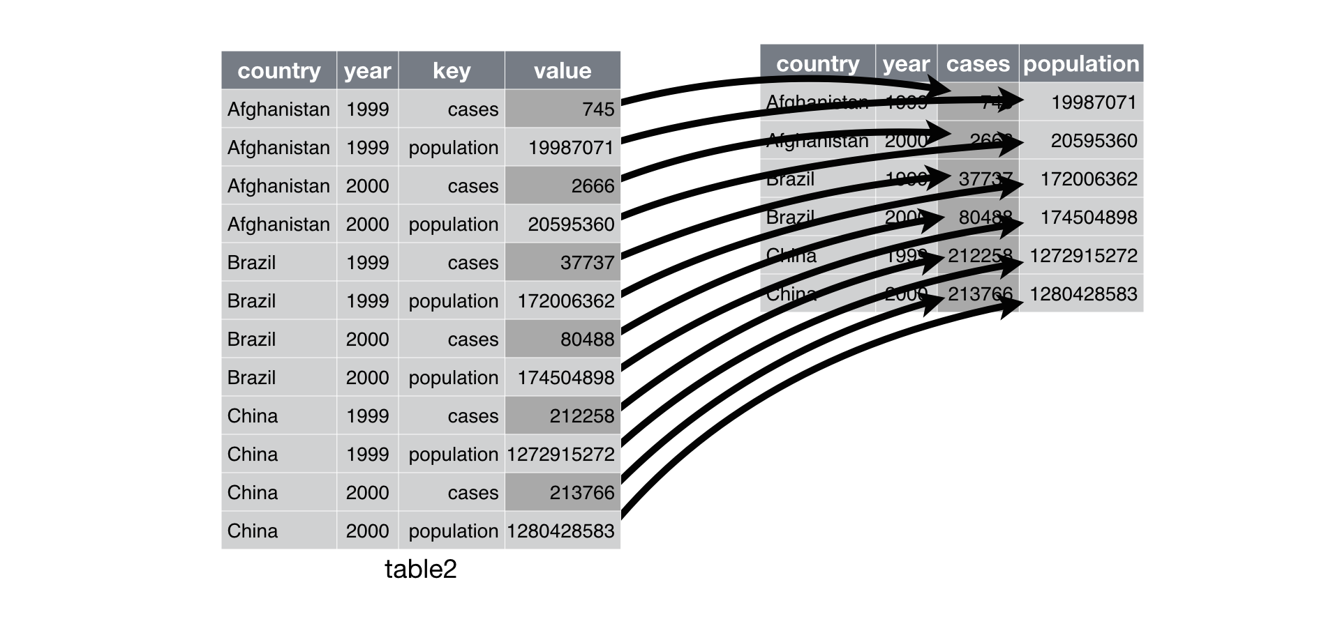

Spreading table2 makes it tidy

gather() makes wide tables narrower and longer

spread() makes long tables shorter and wider

---

Separating and uniting

table3 has a different problem :

one column (rate) that contains two variables (cases and population)

table3

## # A tibble: 6 × 3
##   country      year rate             
## * <chr>       <int> <chr>            
## 1 Afghanistan  1999 745/19987071     
## 2 Afghanistan  2000 2666/20595360    
## 3 Brazil       1999 37737/172006362  
## 4 Brazil       2000 80488/174504898  
## 5 China        1999 212258/1272915272
## 6 China        2000 213766/1280428583

To fix this problem, we will need the separate() function.

The complement of separate() is unite(), to use when a single variable is spread across multiple columns.

---

separate()

This function pulls apart one column into multiple columns, by splitting wherever a separator character appears. Take table3:

table3

## # A tibble: 6 × 3
##   country      year rate             
## * <chr>       <int> <chr>            
## 1 Afghanistan  1999 745/19987071     
## 2 Afghanistan  2000 2666/20595360    
## 3 Brazil       1999 37737/172006362  
## 4 Brazil       2000 80488/174504898  
## 5 China        1999 212258/1272915272
## 6 China        2000 213766/1280428583

The rate column contains both cases and population variables, and we need to split it into two variables.

separate() takes the name of the column to separate, and the names of the columns to separate into, as shown in Figure @ref(fig:tidy-separate) and the code below.

table3 %>% 
  separate(rate, into = c("cases", "population"))

## # A tibble: 6 × 4
##   country      year cases  population
##   <chr>       <int> <chr>  <chr>     
## 1 Afghanistan  1999 745    19987071  
## 2 Afghanistan  2000 2666   20595360  
## 3 Brazil       1999 37737  172006362 
## 4 Brazil       2000 80488  174504898 
## 5 China        1999 212258 1272915272
## 6 China        2000 213766 1280428583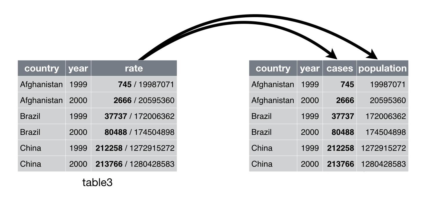

Separating table3 makes it tidy

By default, separate() will split values wherever it sees a non-alphanumeric character.

table3 %>% 
  separate(rate, into = c("cases", "population"), sep = "/")

Look carefully at the column types: you’ll notice that case and population are character columns. This is the default behaviour in separate(): it leaves the type of the column as is. Here, however, it’s not very useful as those really are numbers. We can ask separate() to try and convert to better types using convert = TRUE:

table3 %>% 
  separate(rate, into = c("cases", "population"), convert = TRUE)

## # A tibble: 6 × 4
##   country      year  cases population
##   <chr>       <int>  <int>      <int>
## 1 Afghanistan  1999    745   19987071
## 2 Afghanistan  2000   2666   20595360
## 3 Brazil       1999  37737  172006362
## 4 Brazil       2000  80488  174504898
## 5 China        1999 212258 1272915272
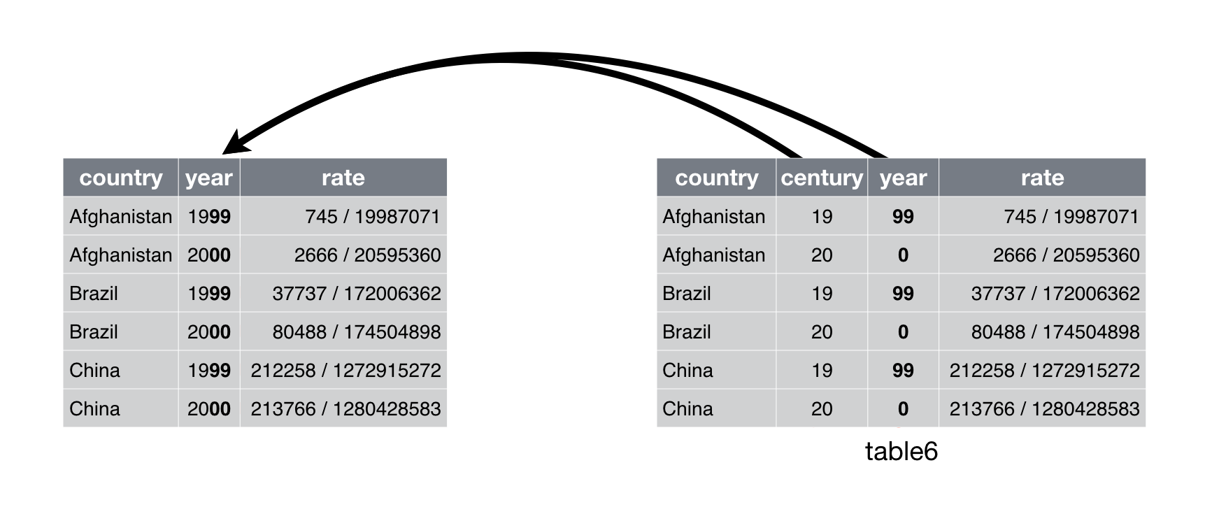
## 6 China        2000 213766 1280428583

You can also pass a vector of integers to sep. separate() will interpret the integers as positions to split at. Positive values start at 1 on the far-left of the strings; negative value start at -1 on the far-right of the strings. When using integers to separate strings, the length of sep should be one less than the number of names in into.

table3 %>% 
  separate(year, into = c("century", "year"), sep = 2)

## # A tibble: 6 × 4
##   country     century year  rate             
##   <chr>       <chr>   <chr> <chr>            
## 1 Afghanistan 19      99    745/19987071     
## 2 Afghanistan 20      00    2666/20595360    
## 3 Brazil      19      99    37737/172006362  
## 4 Brazil      20      00    80488/174504898  
## 5 China       19      99    212258/1272915272
## 6 China       20      00    213766/1280428583

---

unite()

This function is the inverse of separate(): it combines multiple columns into a single column.

Uniting table5 makes it tidy

We can use unite() to rejoin the century and year columns that we created in the last example. That data is saved as tidyr::table5.

table5 %>% 
  unite(new, century, year)

## # A tibble: 6 × 3
##   country     new   rate             
##   <chr>       <chr> <chr>            
## 1 Afghanistan 19_99 745/19987071     
## 2 Afghanistan 20_00 2666/20595360    
## 3 Brazil      19_99 37737/172006362  
## 4 Brazil      20_00 80488/174504898  
## 5 China       19_99 212258/1272915272
## 6 China       20_00 213766/1280428583

In this case we also need to use the sep argument.

The default will place an underscore (_) between the values from different columns.

Here we don’t want any separator so we use "":

table5 %>% 
  unite(new, century, year, sep = "")

## # A tibble: 6 × 3
##   country     new   rate             
##   <chr>       <chr> <chr>            
## 1 Afghanistan 1999  745/19987071     
## 2 Afghanistan 2000  2666/20595360    
## 3 Brazil      1999  37737/172006362  
## 4 Brazil      2000  80488/174504898  
## 5 China       1999  212258/1272915272
## 6 China       2000  213766/1280428583

---

Missing values

Changing the representation of a dataset brings up an important subtlety of missing values.

A value can be missing in one of two possible ways:

• Explicitly –> flagged with NA.

• Implicitly –> simply not present in the data.

Let’s illustrate this idea with a very simple data set:

stocks <- tibble(
  year   = c(2015, 2015, 2015, 2015, 2016, 2016, 2016),
  qtr    = c(   1,    2,    3,    4,    2,    3,    4),
  return = c(1.88, 0.59, 0.35,   NA, 0.92, 0.17, 2.66)
)

print(stocks)

## # A tibble: 7 × 3
##    year   qtr return
##   <dbl> <dbl>  <dbl>
## 1  2015     1   1.88
## 2  2015     2   0.59
## 3  2015     3   0.35
## 4  2015     4  NA   
## 5  2016     2   0.92
## 6  2016     3   0.17
## 7  2016     4   2.66

There are two missing values in this dataset.

We can make the implicit missing value explicit by putting years in the columns:

stocks %>% 
  spread(year, return)

## # A tibble: 4 × 3
##     qtr `2015` `2016`
##   <dbl>  <dbl>  <dbl>
## 1     1   1.88  NA   
## 2     2   0.59   0.92
## 3     3   0.35   0.17
## 4     4  NA      2.66

Because these explicit missing values may not be important in other representations of the data, you can set na.rm = TRUE in gather() to turn explicit missing values implicit:

stocks %>% 
  spread(year, return) %>% 
  gather(year, return, `2015`:`2016`, na.rm = TRUE)

## # A tibble: 6 × 3
##     qtr year  return
##   <dbl> <chr>  <dbl>
## 1     1 2015    1.88
## 2     2 2015    0.59
## 3     3 2015    0.35
## 4     2 2016    0.92
## 5     3 2016    0.17
## 6     4 2016    2.66

Another important tool for making missing values explicit in tidy data is complete():

stocks %>% 
  complete(year, qtr)

## # A tibble: 8 × 3
##    year   qtr return
##   <dbl> <dbl>  <dbl>
## 1  2015     1   1.88
## 2  2015     2   0.59
## 3  2015     3   0.35
## 4  2015     4  NA   
## 5  2016     1  NA   
## 6  2016     2   0.92
## 7  2016     3   0.17
## 8  2016     4   2.66

complete() takes a set of columns, and finds all unique combinations.

It then ensures the original dataset contains all those values, filling in explicit NAs where necessary.

Sometimes when a data source has primarily been used for data entry, missing values indicate that the previous value should be carried forward:

treatment <- tribble(
  ~ person,           ~ treatment, ~response,
  "Derrick Whitmore", 1,           7,
  NA,                 2,           10,
  NA,                 3,           9,
  "Katherine Burke",  1,           4
)

You can fill in these missing values with fill(). It takes a set of columns where you want missing values to be replaced by the most recent non-missing value (sometimes called last observation carried forward).

treatment %>% 
  fill(person)

## # A tibble: 4 × 3
##   person           treatment response
##   <chr>                <dbl>    <dbl>
## 1 Derrick Whitmore         1        7
## 2 Derrick Whitmore         2       10
## 3 Derrick Whitmore         3        9
## 4 Katherine Burke          1        4

---

Case Study

The tidyr::who dataset contains tuberculosis (TB) cases broken down by year, country, age, gender, and diagnosis method.

The data comes from the 2014 World Health Organization Global Tuberculosis Report, available at http://www.who.int/tb/country/data/download/en/.

print(who, n=4)

## # A tibble: 7,240 × 60
##   country iso2  iso3   year new_sp_m014 new_sp_m1524 new_sp_m2534 new_sp_m3544 new_sp_m4554
##   <chr>   <chr> <chr> <int>       <int>        <int>        <int>        <int>        <int>
## 1 Afghan… AF    AFG    1980          NA           NA           NA           NA           NA
## 2 Afghan… AF    AFG    1981          NA           NA           NA           NA           NA
## 3 Afghan… AF    AFG    1982          NA           NA           NA           NA           NA
## 4 Afghan… AF    AFG    1983          NA           NA           NA           NA           NA
## # … with 7,236 more rows, and 51 more variables: new_sp_m5564 <int>, new_sp_m65 <int>,
## #   new_sp_f014 <int>, new_sp_f1524 <int>, new_sp_f2534 <int>, new_sp_f3544 <int>,
## #   new_sp_f4554 <int>, new_sp_f5564 <int>, new_sp_f65 <int>, new_sn_m014 <int>,
## #   new_sn_m1524 <int>, new_sn_m2534 <int>, new_sn_m3544 <int>, new_sn_m4554 <int>,
## #   new_sn_m5564 <int>, new_sn_m65 <int>, new_sn_f014 <int>, new_sn_f1524 <int>,
## #   new_sn_f2534 <int>, new_sn_f3544 <int>, new_sn_f4554 <int>, new_sn_f5564 <int>,
## #   new_sn_f65 <int>, new_ep_m014 <int>, new_ep_m1524 <int>, new_ep_m2534 <int>, …

It contains redundant columns, odd variable codes, and many missing values.

• country, iso2, and iso3 are three variables that redundantly specify the country.

• year is clearly also a variable.

• We don’t know what all the other columns are but given the structure in the variable names (e.g. new_sp_m014, new_ep_m014, new_ep_f014) these are likely to be values, not variables.

So we need to gather() together all the columns from new_sp_m014 to newrel_f65.

We don’t know what those values represent yet, so we’ll give them the generic name "key".

We know the cells represent the count of cases, so we’ll use the variable cases.

There are a lot of missing values in the current representation, so for now we’ll use na.rm just so we can focus on the values that are present.

who1 <- who %>% 
  gather(new_sp_m014:newrel_f65, key = "key", value = "cases", na.rm = TRUE)
who1

## # A tibble: 76,046 × 6
##    country     iso2  iso3   year key         cases
##    <chr>       <chr> <chr> <int> <chr>       <int>
##  1 Afghanistan AF    AFG    1997 new_sp_m014     0
##  2 Afghanistan AF    AFG    1998 new_sp_m014    30
##  3 Afghanistan AF    AFG    1999 new_sp_m014     8
##  4 Afghanistan AF    AFG    2000 new_sp_m014    52
##  5 Afghanistan AF    AFG    2001 new_sp_m014   129
##  6 Afghanistan AF    AFG    2002 new_sp_m014    90
##  7 Afghanistan AF    AFG    2003 new_sp_m014   127
##  8 Afghanistan AF    AFG    2004 new_sp_m014   139
##  9 Afghanistan AF    AFG    2005 new_sp_m014   151
## 10 Afghanistan AF    AFG    2006 new_sp_m014   193
## # … with 76,036 more rows

We can get some hint of the structure of the values in the new key column by counting them:

who1 %>% 
  count(key)

## # A tibble: 56 × 2
##    key              n
##    <chr>        <int>
##  1 new_ep_f014   1032
##  2 new_ep_f1524  1021
##  3 new_ep_f2534  1021
##  4 new_ep_f3544  1021
##  5 new_ep_f4554  1017
##  6 new_ep_f5564  1017
##  7 new_ep_f65    1014
##  8 new_ep_m014   1038
##  9 new_ep_m1524  1026
## 10 new_ep_m2534  1020
## # … with 46 more rows

It tells us:

1. The first three letters of each column denote whether the column contains new or old cases of TB. In this dataset, each column contains new cases.

2. The next two letters describe the type of TB:

   • rel stands for cases of relapse
   • ep stands for cases of extrapulmonary TB
   • sn stands for cases of pulmonary TB that could not be diagnosed by a pulmonary smear (smear negative)
   • sp stands for cases of pulmonary TB that could be diagnosed be a pulmonary smear (smear positive)

3. The sixth letter gives the sex of TB patients. The dataset groups cases by males (m) and females (f).

4. The remaining numbers gives the age group. The dataset groups cases into seven age groups:

   • 014 = 0 – 14 years old
   • 1524 = 15 – 24 years old
   • 2534 = 25 – 34 years old
   • …
   • 65 = 65 or older

We need to make a minor fix to the format of the column names.

who2 <- who1 %>% 
  mutate(key = stringr::str_replace(key, "newrel", "new_rel"))
who2

## # A tibble: 76,046 × 6
##    country     iso2  iso3   year key         cases
##    <chr>       <chr> <chr> <int> <chr>       <int>
##  1 Afghanistan AF    AFG    1997 new_sp_m014     0
##  2 Afghanistan AF    AFG    1998 new_sp_m014    30
##  3 Afghanistan AF    AFG    1999 new_sp_m014     8
##  4 Afghanistan AF    AFG    2000 new_sp_m014    52
##  5 Afghanistan AF    AFG    2001 new_sp_m014   129
##  6 Afghanistan AF    AFG    2002 new_sp_m014    90
##  7 Afghanistan AF    AFG    2003 new_sp_m014   127
##  8 Afghanistan AF    AFG    2004 new_sp_m014   139
##  9 Afghanistan AF    AFG    2005 new_sp_m014   151
## 10 Afghanistan AF    AFG    2006 new_sp_m014   193
## # … with 76,036 more rows

We can separate the values in each code with two passes of separate().

who3 <- who2 %>% 
  separate(key, c("new", "type", "sexage"), sep = "_")
who3

## # A tibble: 76,046 × 8
##    country     iso2  iso3   year new   type  sexage cases
##    <chr>       <chr> <chr> <int> <chr> <chr> <chr>  <int>
##  1 Afghanistan AF    AFG    1997 new   sp    m014       0
##  2 Afghanistan AF    AFG    1998 new   sp    m014      30
##  3 Afghanistan AF    AFG    1999 new   sp    m014       8
##  4 Afghanistan AF    AFG    2000 new   sp    m014      52
##  5 Afghanistan AF    AFG    2001 new   sp    m014     129
##  6 Afghanistan AF    AFG    2002 new   sp    m014      90
##  7 Afghanistan AF    AFG    2003 new   sp    m014     127
##  8 Afghanistan AF    AFG    2004 new   sp    m014     139
##  9 Afghanistan AF    AFG    2005 new   sp    m014     151
## 10 Afghanistan AF    AFG    2006 new   sp    m014     193
## # … with 76,036 more rows

Then we might as well drop the new column because it’s constant in this dataset. While we’re dropping columns, let’s also drop iso2 and iso3 since they’re redundant.

who3 %>% 
  count(new)

## # A tibble: 1 × 2
##   new       n
##   <chr> <int>
## 1 new   76046

who4 <- who3 %>% 
  select(-new, -iso2, -iso3)

Next we’ll separate sexage into sex and age by splitting after the first character:

who5 <- who4 %>% 
  separate(sexage, c("sex", "age"), sep = 1)
print(who5, n=5)

## # A tibble: 76,046 × 6
##   country      year type  sex   age   cases
##   <chr>       <int> <chr> <chr> <chr> <int>
## 1 Afghanistan  1997 sp    m     014       0
## 2 Afghanistan  1998 sp    m     014      30
## 3 Afghanistan  1999 sp    m     014       8
## 4 Afghanistan  2000 sp    m     014      52
## 5 Afghanistan  2001 sp    m     014     129
## # … with 76,041 more rows

A work by Matteo Cereda and Fabio Iannelli